3.2 Window Functions
Warning
Prior to version 0.18.0, pd.rolling_*, pd.expanding_*, and pd.ewm* were module level
functions and are now deprecated. These are replaced by using the Rolling, Expanding and EWM. objects and a corresponding method call.
The deprecation warning will show the new syntax, see an example here You can view the previous documentation here
For working with data, a number of windows functions are provided for computing common window or rolling statistics. Among these are count, sum, mean, median, correlation, variance, covariance, standard deviation, skewness, and kurtosis.
Note
The API for window statistics is quite similar to the way one works with GroupBy objects, see the documentation here
We work with rolling, expanding and exponentially weighted data through the corresponding
objects, Rolling, Expanding and EWM.
In [1]: s = pd.Series(np.random.randn(1000), index=pd.date_range('1/1/2000', periods=1000))

In [2]: s = s.cumsum()

In [3]: s
Out[3]:
2000-01-01     0.469112
2000-01-02     0.186249
2000-01-03    -1.322810
2000-01-04    -2.458442
                ...
2002-09-23   -44.645728
2002-09-24   -44.953742
2002-09-25   -45.033657
2002-09-26   -46.044246
Freq: D, dtype: float64
These are created from methods on Series and DataFrame.
In [4]: r = s.rolling(window=60)

In [5]: r
Out[5]: Rolling [window=60,center=False,axis=0]
These object provide tab-completion of the avaible methods and properties.
In [14]: r.
r.agg         r.apply       r.count       r.exclusions  r.max         r.median      r.name        r.skew        r.sum
r.aggregate   r.corr        r.cov         r.kurt        r.mean        r.min         r.quantile    r.std         r.var
Generally these methods all have the same interface. They all accept the following arguments:
window: size of moving windowmin_periods: threshold of non-null data points to require (otherwise result is NA)center: boolean, whether to set the labels at the center (default is False)
Warning
The freq and how arguments were in the API prior to 0.18.0 changes. These are deprecated in the new API. You can simply resample the input prior to creating a window function.
For example, instead of s.rolling(window=5,freq='D').max() to get the max value on a rolling 5 Day window, one could use s.resample('D').max().rolling(window=5).max(), which first resamples the data to daily data, then provides a rolling 5 day window.
We can then call methods on these rolling objects. These return like-indexed objects:
In [6]: r.mean()
Out[6]:
2000-01-01          NaN
2000-01-02          NaN
2000-01-03          NaN
2000-01-04          NaN
                ...
2002-09-23   -40.090910
2002-09-24   -40.187383
2002-09-25   -40.285841
2002-09-26   -40.404663
Freq: D, dtype: float64
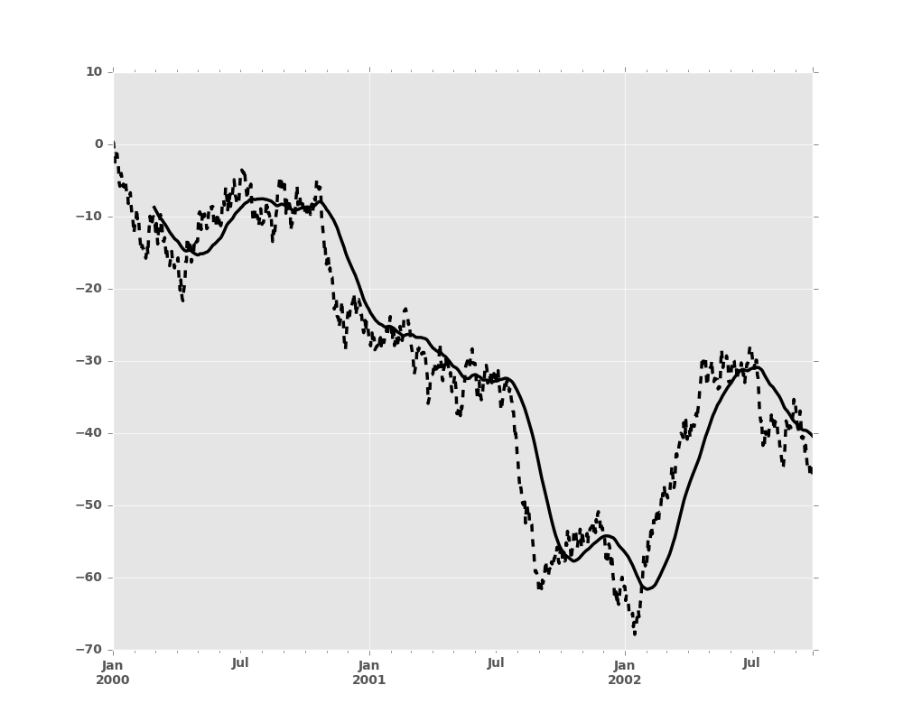
In [7]: s.plot(style='k--')
Out[7]: <matplotlib.axes._subplots.AxesSubplot at 0x2b35acae3a10>

In [8]: r.mean().plot(style='k')
Out[8]: <matplotlib.axes._subplots.AxesSubplot at 0x2b35acae3a10>
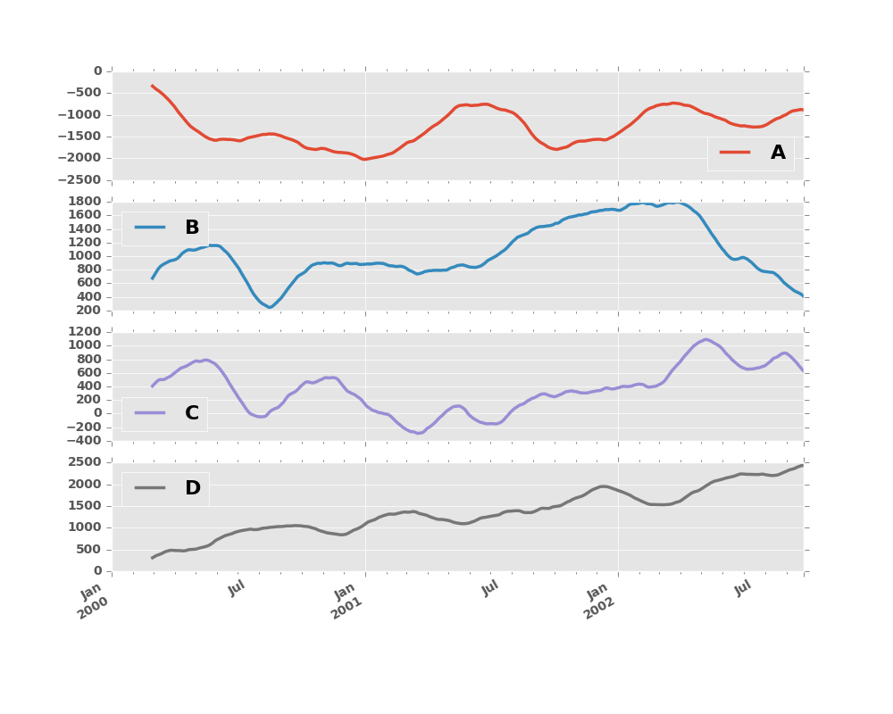
They can also be applied to DataFrame objects. This is really just syntactic sugar for applying the moving window operator to all of the DataFrame’s columns:
In [9]: df = pd.DataFrame(np.random.randn(1000, 4),
   ...:                   index=pd.date_range('1/1/2000', periods=1000),
   ...:                   columns=['A', 'B', 'C', 'D'])
   ...:

In [10]: df = df.cumsum()

In [11]: df.rolling(window=60).sum().plot(subplots=True)
Out[11]:
array([<matplotlib.axes._subplots.AxesSubplot object at 0x2b35acd7e090>,
       <matplotlib.axes._subplots.AxesSubplot object at 0x2b35ace33b50>,
       <matplotlib.axes._subplots.AxesSubplot object at 0x2b35aceb5f90>,
       <matplotlib.axes._subplots.AxesSubplot object at 0x2b35acf17e50>], dtype=object)
3.2.1 Method Summary
We provide a number of the common statistical functions:
| Method | Description |
|---|---|
count() |
Number of non-null observations |
sum() |
Sum of values |
mean() |
Mean of values |
median() |
Arithmetic median of values |
min() |
Minimum |
max() |
Maximum |
std() |
Bessel-corrected sample standard deviation |
var() |
Unbiased variance |
skew() |
Sample skewness (3rd moment) |
kurt() |
Sample kurtosis (4th moment) |
quantile() |
Sample quantile (value at %) |
apply() |
Generic apply |
cov() |
Unbiased covariance (binary) |
corr() |
Correlation (binary) |
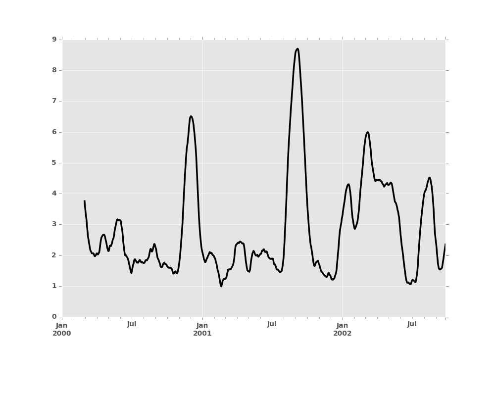
The apply() function takes an extra func argument and performs
generic rolling computations. The func argument should be a single function
that produces a single value from an ndarray input. Suppose we wanted to
compute the mean absolute deviation on a rolling basis:
In [12]: mad = lambda x: np.fabs(x - x.mean()).mean()

In [13]: s.rolling(window=60).apply(mad).plot(style='k')
Out[13]: <matplotlib.axes._subplots.AxesSubplot at 0x2b35acbb5e50>
3.2.2 Rolling Windows
Passing win_type to .rolling generates a generic rolling window computation, that is weighted according the win_type.
The following methods are available:
| Method | Description |
|---|---|
sum() |
Sum of values |
mean() |
Mean of values |
The weights used in the window are specified by the win_type keyword. The list of recognized types are:
boxcartriangblackmanhammingbartlettparzenbohmanblackmanharrisnuttallbarthannkaiser(needs beta)gaussian(needs std)general_gaussian(needs power, width)slepian(needs width).
In [14]: ser = pd.Series(np.random.randn(10), index=pd.date_range('1/1/2000', periods=10))

In [15]: ser.rolling(window=5, win_type='triang').mean()
Out[15]:
2000-01-01         NaN
2000-01-02         NaN
2000-01-03         NaN
2000-01-04         NaN
                ...
2000-01-07    0.444733
2000-01-08    0.479115
2000-01-09    0.184728
2000-01-10    0.215758
Freq: D, dtype: float64
Note that the boxcar window is equivalent to mean().
In [16]: ser.rolling(window=5, win_type='boxcar').mean()
Out[16]:
2000-01-01         NaN
2000-01-02         NaN
2000-01-03         NaN
2000-01-04         NaN
                ...
2000-01-07   -0.018978
2000-01-08    0.400008
2000-01-09    0.539270
2000-01-10    0.153939
Freq: D, dtype: float64

In [17]: ser.rolling(window=5).mean()
Out[17]:
2000-01-01         NaN
2000-01-02         NaN
2000-01-03         NaN
2000-01-04         NaN
                ...
2000-01-07   -0.018978
2000-01-08    0.400008
2000-01-09    0.539270
2000-01-10    0.153939
Freq: D, dtype: float64
For some windowing functions, additional parameters must be specified:
In [18]: ser.rolling(window=5, win_type='gaussian').mean(std=0.1)
Out[18]:
2000-01-01         NaN
2000-01-02         NaN
2000-01-03         NaN
2000-01-04         NaN
                ...
2000-01-07    1.636865
2000-01-08    1.248347
2000-01-09   -1.821568
2000-01-10    1.360994
Freq: D, dtype: float64
Note
For .sum() with a win_type, there is no normalization done to the
weights for the window. Passing custom weights of [1, 1, 1] will yield a different
result than passing weights of [2, 2, 2], for example. When passing a
win_type instead of explicitly specifying the weights, the weights are
already normalized so that the largest weight is 1.
In contrast, the nature of the .mean() calculation is
such that the weights are normalized with respect to each other. Weights
of [1, 1, 1] and [2, 2, 2] yield the same result.
3.2.3 Time-aware Rolling
New in version 0.19.0.
New in version 0.19.0 are the ability to pass an offset (or convertible) to a .rolling() method and have it produce
variable sized windows based on the passed time window. For each time point, this includes all preceding values occurring
within the indicated time delta.
This can be particularly useful for a non-regular time frequency index.
In [19]: dft = pd.DataFrame({'B': [0, 1, 2, np.nan, 4]},
   ....:                    index=pd.date_range('20130101 09:00:00', periods=5, freq='s'))
   ....:

In [20]: dft
Out[20]:
                       B
2013-01-01 09:00:00  0.0
2013-01-01 09:00:01  1.0
2013-01-01 09:00:02  2.0
2013-01-01 09:00:03  NaN
2013-01-01 09:00:04  4.0
This is a regular frequency index. Using an integer window parameter works to roll along the window frequency.
In [21]: dft.rolling(2).sum()
Out[21]:
                       B
2013-01-01 09:00:00  NaN
2013-01-01 09:00:01  1.0
2013-01-01 09:00:02  3.0
2013-01-01 09:00:03  NaN
2013-01-01 09:00:04  NaN

In [22]: dft.rolling(2, min_periods=1).sum()
Out[22]:
                       B
2013-01-01 09:00:00  0.0
2013-01-01 09:00:01  1.0
2013-01-01 09:00:02  3.0
2013-01-01 09:00:03  2.0
2013-01-01 09:00:04  4.0
Specifying an offset allows a more intuitive specification of the rolling frequency.
In [23]: dft.rolling('2s').sum()
Out[23]:
                       B
2013-01-01 09:00:00  0.0
2013-01-01 09:00:01  1.0
2013-01-01 09:00:02  3.0
2013-01-01 09:00:03  2.0
2013-01-01 09:00:04  4.0
Using a non-regular, but still monotonic index, rolling with an integer window does not impart any special calculation.
In [24]: dft = pd.DataFrame({'B': [0, 1, 2, np.nan, 4]},
   ....:                    index = pd.Index([pd.Timestamp('20130101 09:00:00'),
   ....:                                      pd.Timestamp('20130101 09:00:02'),
   ....:                                      pd.Timestamp('20130101 09:00:03'),
   ....:                                      pd.Timestamp('20130101 09:00:05'),
   ....:                                      pd.Timestamp('20130101 09:00:06')],
   ....:                                     name='foo'))
   ....:

In [25]: dft
Out[25]:
                       B
foo
2013-01-01 09:00:00  0.0
2013-01-01 09:00:02  1.0
2013-01-01 09:00:03  2.0
2013-01-01 09:00:05  NaN
2013-01-01 09:00:06  4.0

In [26]: dft.rolling(2).sum()
Out[26]:
                       B
foo
2013-01-01 09:00:00  NaN
2013-01-01 09:00:02  1.0
2013-01-01 09:00:03  3.0
2013-01-01 09:00:05  NaN
2013-01-01 09:00:06  NaN
Using the time-specification generates variable windows for this sparse data.
In [27]: dft.rolling('2s').sum()
Out[27]:
                       B
foo
2013-01-01 09:00:00  0.0
2013-01-01 09:00:02  1.0
2013-01-01 09:00:03  3.0
2013-01-01 09:00:05  NaN
2013-01-01 09:00:06  4.0
Furthermore, we now allow an optional on parameter to specify a column (rather than the
default of the index) in a DataFrame.
In [28]: dft = dft.reset_index()

In [29]: dft
Out[29]:
                  foo    B
0 2013-01-01 09:00:00  0.0
1 2013-01-01 09:00:02  1.0
2 2013-01-01 09:00:03  2.0
3 2013-01-01 09:00:05  NaN
4 2013-01-01 09:00:06  4.0

In [30]: dft.rolling('2s', on='foo').sum()
Out[30]:
                  foo    B
0 2013-01-01 09:00:00  0.0
1 2013-01-01 09:00:02  1.0
2 2013-01-01 09:00:03  3.0
3 2013-01-01 09:00:05  NaN
4 2013-01-01 09:00:06  4.0
3.2.4 Time-aware Rolling vs. Resampling
Using .rolling() with a time-based index is quite similar to resampling. They
both operate and perform reductive operations on time-indexed pandas objects.
When using .rolling() with an offset. The offset is a time-delta. Take a backwards-in-time looking window, and
aggregate all of the values in that window (including the end-point, but not the start-point). This is the new value
at that point in the result. These are variable sized windows in time-space for each point of the input. You will get
a same sized result as the input.
When using .resample() with an offset. Construct a new index that is the frequency of the offset. For each frequency
bin, aggregate points from the input within a backwards-in-time looking window that fall in that bin. The result of this
aggregation is the output for that frequency point. The windows are fixed size size in the frequency space. Your result
will have the shape of a regular frequency between the min and the max of the original input object.
To summarize, .rolling() is a time-based window operation, while .resample() is a frequency-based window operation.
3.2.5 Centering Windows
By default the labels are set to the right edge of the window, but a
center keyword is available so the labels can be set at the center.
In [31]: ser.rolling(window=5).mean()
Out[31]:
2000-01-01         NaN
2000-01-02         NaN
2000-01-03         NaN
2000-01-04         NaN
                ...
2000-01-07   -0.018978
2000-01-08    0.400008
2000-01-09    0.539270
2000-01-10    0.153939
Freq: D, dtype: float64

In [32]: ser.rolling(window=5, center=True).mean()
Out[32]:
2000-01-01         NaN
2000-01-02         NaN
2000-01-03    0.386370
2000-01-04    0.460074
                ...
2000-01-07    0.539270
2000-01-08    0.153939
2000-01-09         NaN
2000-01-10         NaN
Freq: D, dtype: float64
3.2.6 Binary Window Functions
cov() and corr() can compute moving window statistics about
two Series or any combination of DataFrame/Series or
DataFrame/DataFrame. Here is the behavior in each case:
- two
Series: compute the statistic for the pairing. DataFrame/Series: compute the statistics for each column of the DataFrame with the passed Series, thus returning a DataFrame.DataFrame/DataFrame: by default compute the statistic for matching column names, returning a DataFrame. If the keyword argumentpairwise=Trueis passed then computes the statistic for each pair of columns, returning aPanelwhoseitemsare the dates in question (see the next section).
For example:
In [33]: df2 = df[:20]

In [34]: df2.rolling(window=5).corr(df2['B'])
Out[34]:
                   A    B         C         D
2000-01-01       NaN  NaN       NaN       NaN
2000-01-02       NaN  NaN       NaN       NaN
2000-01-03       NaN  NaN       NaN       NaN
2000-01-04       NaN  NaN       NaN       NaN
...              ...  ...       ...       ...
2000-01-17  0.245266  1.0 -0.828150 -0.580157
2000-01-18  0.447883  1.0 -0.901636  0.907240
2000-01-19 -0.140933  1.0  0.164937  0.956559
2000-01-20 -0.666317  1.0 -0.324339  0.968124

[20 rows x 4 columns]
3.2.7 Computing rolling pairwise covariances and correlations
In financial data analysis and other fields it’s common to compute covariance
and correlation matrices for a collection of time series. Often one is also
interested in moving-window covariance and correlation matrices. This can be
done by passing the pairwise keyword argument, which in the case of
DataFrame inputs will yield a Panel whose items are the dates in
question. In the case of a single DataFrame argument the pairwise argument
can even be omitted:
Note
Missing values are ignored and each entry is computed using the pairwise complete observations. Please see the covariance section for caveats associated with this method of calculating covariance and correlation matrices.
In [35]: covs = df[['B','C','D']].rolling(window=50).cov(df[['A','B','C']], pairwise=True)

In [36]: covs[df.index[-50]]
Out[36]:
          A          B          C
B -9.024783  21.812311 -10.328820
C  4.689587 -10.328820   8.037580
D  1.481747   0.785067  -0.840609
In [37]: correls = df.rolling(window=50).corr()

In [38]: correls[df.index[-50]]
Out[38]:
          A         B         C         D
A  1.000000 -0.579381  0.495964  0.363033
B -0.579381  1.000000 -0.780077  0.137356
C  0.495964 -0.780077  1.000000 -0.242284
D  0.363033  0.137356 -0.242284  1.000000
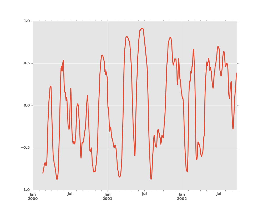
You can efficiently retrieve the time series of correlations between two
columns using .loc indexing:
In [39]: correls.loc[:, 'A', 'C'].plot()
Out[39]: <matplotlib.axes._subplots.AxesSubplot at 0x2b35b9c0de50>