2 DataFrame
DataFrame is a 2-dimensional labeled data structure with columns of potentially different types. You can think of it like a spreadsheet or SQL table, or a dict of Series objects. It is generally the most commonly used pandas object. Like Series, DataFrame accepts many different kinds of input:
- Dict of 1D ndarrays, lists, dicts, or Series
- 2-D numpy.ndarray
- Structured or record ndarray
- A
Series- Another
DataFrame
Along with the data, you can optionally pass index (row labels) and columns (column labels) arguments. If you pass an index and / or columns, you are guaranteeing the index and / or columns of the resulting DataFrame. Thus, a dict of Series plus a specific index will discard all data not matching up to the passed index.
If axis labels are not passed, they will be constructed from the input data based on common sense rules.
2.1 From dict of Series or dicts
The result index will be the union of the indexes of the various Series. If there are any nested dicts, these will be first converted to Series. If no columns are passed, the columns will be the sorted list of dict keys.
In [1]: d = {'one' : pd.Series([1., 2., 3.], index=['a', 'b', 'c']),
   ...:      'two' : pd.Series([1., 2., 3., 4.], index=['a', 'b', 'c', 'd'])}
   ...:

In [2]: df = pd.DataFrame(d)

In [3]: df
Out[3]:
   one  two
a  1.0  1.0
b  2.0  2.0
c  3.0  3.0
d  NaN  4.0

In [4]: pd.DataFrame(d, index=['d', 'b', 'a'])
Out[4]:
   one  two
d  NaN  4.0
b  2.0  2.0
a  1.0  1.0

In [5]: pd.DataFrame(d, index=['d', 'b', 'a'], columns=['two', 'three'])
Out[5]:
   two three
d  4.0   NaN
b  2.0   NaN
a  1.0   NaN
The row and column labels can be accessed respectively by accessing the index and columns attributes:
Note
When a particular set of columns is passed along with a dict of data, the passed columns override the keys in the dict.
In [6]: df.index
Out[6]: Index([u'a', u'b', u'c', u'd'], dtype='object')

In [7]: df.columns
Out[7]: Index([u'one', u'two'], dtype='object')
2.2 From dict of ndarrays / lists
The ndarrays must all be the same length. If an index is passed, it must
clearly also be the same length as the arrays. If no index is passed, the
result will be range(n), where n is the array length.
In [8]: d = {'one' : [1., 2., 3., 4.],
   ...:      'two' : [4., 3., 2., 1.]}
   ...:

In [9]: pd.DataFrame(d)
Out[9]:
   one  two
0  1.0  4.0
1  2.0  3.0
2  3.0  2.0
3  4.0  1.0

In [10]: pd.DataFrame(d, index=['a', 'b', 'c', 'd'])
Out[10]:
   one  two
a  1.0  4.0
b  2.0  3.0
c  3.0  2.0
d  4.0  1.0
2.3 From structured or record array
This case is handled identically to a dict of arrays.
In [11]: data = np.zeros((2,), dtype=[('A', 'i4'),('B', 'f4'),('C', 'a10')])

In [12]: data[:] = [(1,2.,'Hello'), (2,3.,"World")]

In [13]: pd.DataFrame(data)
Out[13]:
   A    B      C
0  1  2.0  Hello
1  2  3.0  World

In [14]: pd.DataFrame(data, index=['first', 'second'])
Out[14]:
        A    B      C
first   1  2.0  Hello
second  2  3.0  World

In [15]: pd.DataFrame(data, columns=['C', 'A', 'B'])
Out[15]:
       C  A    B
0  Hello  1  2.0
1  World  2  3.0
Note
DataFrame is not intended to work exactly like a 2-dimensional NumPy ndarray.
2.4 From a list of dicts
In [16]: data2 = [{'a': 1, 'b': 2}, {'a': 5, 'b': 10, 'c': 20}]

In [17]: pd.DataFrame(data2)
Out[17]:
   a   b     c
0  1   2   NaN
1  5  10  20.0

In [18]: pd.DataFrame(data2, index=['first', 'second'])
Out[18]:
        a   b     c
first   1   2   NaN
second  5  10  20.0

In [19]: pd.DataFrame(data2, columns=['a', 'b'])
Out[19]:
   a   b
0  1   2
1  5  10
2.5 From a dict of tuples
You can automatically create a multi-indexed frame by passing a tuples dictionary
In [20]: pd.DataFrame({('a', 'b'): {('A', 'B'): 1, ('A', 'C'): 2},
   ....:               ('a', 'a'): {('A', 'C'): 3, ('A', 'B'): 4},
   ....:               ('a', 'c'): {('A', 'B'): 5, ('A', 'C'): 6},
   ....:               ('b', 'a'): {('A', 'C'): 7, ('A', 'B'): 8},
   ....:               ('b', 'b'): {('A', 'D'): 9, ('A', 'B'): 10}})
   ....:
Out[20]:
       a              b
       a    b    c    a     b
A B  4.0  1.0  5.0  8.0  10.0
  C  3.0  2.0  6.0  7.0   NaN
  D  NaN  NaN  NaN  NaN   9.0
2.6 From a Series
The result will be a DataFrame with the same index as the input Series, and with one column whose name is the original name of the Series (only if no other column name provided).
Missing Data
Much more will be said on this topic in the Missing data
section. To construct a DataFrame with missing data, use np.nan for those
values which are missing. Alternatively, you may pass a numpy.MaskedArray
as the data argument to the DataFrame constructor, and its masked entries will
be considered missing.
2.7 Alternate Constructors
DataFrame.from_dict
DataFrame.from_dict takes a dict of dicts or a dict of array-like sequences
and returns a DataFrame. It operates like the DataFrame constructor except
for the orient parameter which is 'columns' by default, but which can be
set to 'index' in order to use the dict keys as row labels.
DataFrame.from_records
DataFrame.from_records takes a list of tuples or an ndarray with structured
dtype. Works analogously to the normal DataFrame constructor, except that
index maybe be a specific field of the structured dtype to use as the index.
For example:
In [21]: data
Out[21]:
array([(1, 2.0, 'Hello'), (2, 3.0, 'World')],
      dtype=[('A', '<i4'), ('B', '<f4'), ('C', 'S10')])

In [22]: pd.DataFrame.from_records(data, index='C')
Out[22]:
       A    B
C
Hello  1  2.0
World  2  3.0
DataFrame.from_items
DataFrame.from_items works analogously to the form of the dict
constructor that takes a sequence of (key, value) pairs, where the keys are
column (or row, in the case of orient='index') names, and the value are the
column values (or row values). This can be useful for constructing a DataFrame
with the columns in a particular order without having to pass an explicit list
of columns:
In [23]: pd.DataFrame.from_items([('A', [1, 2, 3]), ('B', [4, 5, 6])])
Out[23]:
   A  B
0  1  4
1  2  5
2  3  6
If you pass orient='index', the keys will be the row labels. But in this
case you must also pass the desired column names:
In [24]: pd.DataFrame.from_items([('A', [1, 2, 3]), ('B', [4, 5, 6])],
   ....:                         orient='index', columns=['one', 'two', 'three'])
   ....:
Out[24]:
   one  two  three
A    1    2      3
B    4    5      6
2.8 Column selection, addition, deletion
You can treat a DataFrame semantically like a dict of like-indexed Series objects. Getting, setting, and deleting columns works with the same syntax as the analogous dict operations:
In [25]: df['one']
Out[25]:
a    1.0
b    2.0
c    3.0
d    NaN
Name: one, dtype: float64

In [26]: df['three'] = df['one'] * df['two']

In [27]: df['flag'] = df['one'] > 2

In [28]: df
Out[28]:
   one  two  three   flag
a  1.0  1.0    1.0  False
b  2.0  2.0    4.0  False
c  3.0  3.0    9.0   True
d  NaN  4.0    NaN  False
Columns can be deleted or popped like with a dict:
In [29]: del df['two']

In [30]: three = df.pop('three')

In [31]: df
Out[31]:
   one   flag
a  1.0  False
b  2.0  False
c  3.0   True
d  NaN  False
When inserting a scalar value, it will naturally be propagated to fill the column:
In [32]: df['foo'] = 'bar'

In [33]: df
Out[33]:
   one   flag  foo
a  1.0  False  bar
b  2.0  False  bar
c  3.0   True  bar
d  NaN  False  bar
When inserting a Series that does not have the same index as the DataFrame, it will be conformed to the DataFrame’s index:
In [34]: df['one_trunc'] = df['one'][:2]

In [35]: df
Out[35]:
   one   flag  foo  one_trunc
a  1.0  False  bar        1.0
b  2.0  False  bar        2.0
c  3.0   True  bar        NaN
d  NaN  False  bar        NaN
You can insert raw ndarrays but their length must match the length of the DataFrame’s index.
By default, columns get inserted at the end. The insert function is
available to insert at a particular location in the columns:
In [36]: df.insert(1, 'bar', df['one'])

In [37]: df
Out[37]:
   one  bar   flag  foo  one_trunc
a  1.0  1.0  False  bar        1.0
b  2.0  2.0  False  bar        2.0
c  3.0  3.0   True  bar        NaN
d  NaN  NaN  False  bar        NaN
2.9 Assigning New Columns in Method Chains
New in version 0.16.0.
Inspired by dplyr’s
mutate verb, DataFrame has an assign()
method that allows you to easily create new columns that are potentially
derived from existing columns.
In [38]: iris = pd.read_csv('https://raw.githubusercontent.com/pydata/pandas/master/doc/data/iris.data')

In [39]: iris.head()
Out[39]:
   SepalLength  SepalWidth  PetalLength  PetalWidth         Name
0          5.1         3.5          1.4         0.2  Iris-setosa
1          4.9         3.0          1.4         0.2  Iris-setosa
2          4.7         3.2          1.3         0.2  Iris-setosa
3          4.6         3.1          1.5         0.2  Iris-setosa
4          5.0         3.6          1.4         0.2  Iris-setosa

In [40]: (iris.assign(sepal_ratio = iris['SepalWidth'] / iris['SepalLength'])
   ....:      .head())
   ....:
Out[40]:
   SepalLength  SepalWidth  PetalLength  PetalWidth         Name  sepal_ratio
0          5.1         3.5          1.4         0.2  Iris-setosa       0.6863
1          4.9         3.0          1.4         0.2  Iris-setosa       0.6122
2          4.7         3.2          1.3         0.2  Iris-setosa       0.6809
3          4.6         3.1          1.5         0.2  Iris-setosa       0.6739
4          5.0         3.6          1.4         0.2  Iris-setosa       0.7200
Above was an example of inserting a precomputed value. We can also pass in a function of one argument to be evalutated on the DataFrame being assigned to.
In [41]: iris.assign(sepal_ratio = lambda x: (x['SepalWidth'] /
   ....:                                      x['SepalLength'])).head()
   ....:
Out[41]:
   SepalLength  SepalWidth  PetalLength  PetalWidth         Name  sepal_ratio
0          5.1         3.5          1.4         0.2  Iris-setosa       0.6863
1          4.9         3.0          1.4         0.2  Iris-setosa       0.6122
2          4.7         3.2          1.3         0.2  Iris-setosa       0.6809
3          4.6         3.1          1.5         0.2  Iris-setosa       0.6739
4          5.0         3.6          1.4         0.2  Iris-setosa       0.7200
assign always returns a copy of the data, leaving the original
DataFrame untouched.
Passing a callable, as opposed to an actual value to be inserted, is
useful when you don’t have a reference to the DataFrame at hand. This is
common when using assign in chains of operations. For example,
we can limit the DataFrame to just those observations with a Sepal Length
greater than 5, calculate the ratio, and plot:
In [42]: (iris.query('SepalLength > 5')
   ....:      .assign(SepalRatio = lambda x: x.SepalWidth / x.SepalLength,
   ....:              PetalRatio = lambda x: x.PetalWidth / x.PetalLength)
   ....:      .plot(kind='scatter', x='SepalRatio', y='PetalRatio'))
   ....:
Out[42]: <matplotlib.axes._subplots.AxesSubplot at 0x2b35ba0c5cd0>
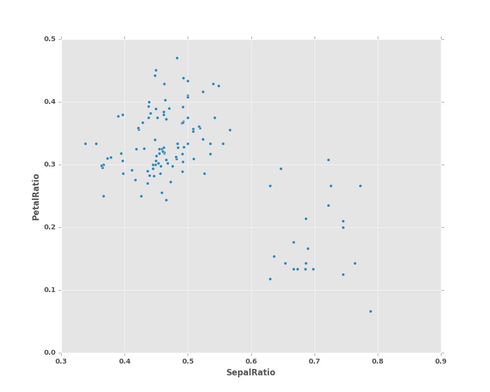
Since a function is passed in, the function is computed on the DataFrame being assigned to. Importantly, this is the DataFrame that’s been filtered to those rows with sepal length greater than 5. The filtering happens first, and then the ratio calculations. This is an example where we didn’t have a reference to the filtered DataFrame available.
The function signature for assign is simply **kwargs. The keys
are the column names for the new fields, and the values are either a value
to be inserted (for example, a Series or NumPy array), or a function
of one argument to be called on the DataFrame. A copy of the original
DataFrame is returned, with the new values inserted.
Warning
Since the function signature of assign is **kwargs, a dictionary,
the order of the new columns in the resulting DataFrame cannot be guaranteed
to match the order you pass in. To make things predictable, items are inserted
alphabetically (by key) at the end of the DataFrame.
All expressions are computed first, and then assigned. So you can’t refer
to another column being assigned in the same call to assign. For example:
In [43]: # Don't do this, bad reference to `C`
        df.assign(C = lambda x: x['A'] + x['B'],
                  D = lambda x: x['A'] + x['C'])
In [2]: # Instead, break it into two assigns
        (df.assign(C = lambda x: x['A'] + x['B'])
           .assign(D = lambda x: x['A'] + x['C']))
2.10 Indexing / Selection
The basics of indexing are as follows:
| Operation | Syntax | Result |
|---|---|---|
| Select column | df[col] |
Series |
| Select row by label | df.loc[label] |
Series |
| Select row by integer location | df.iloc[loc] |
Series |
| Slice rows | df[5:10] |
DataFrame |
| Select rows by boolean vector | df[bool_vec] |
DataFrame |
Row selection, for example, returns a Series whose index is the columns of the DataFrame:
In [44]: df.loc['b']
Out[44]:
one              2
bar              2
flag         False
foo            bar
one_trunc        2
Name: b, dtype: object

In [45]: df.iloc[2]
Out[45]:
one             3
bar             3
flag         True
foo           bar
one_trunc     NaN
Name: c, dtype: object
For a more exhaustive treatment of more sophisticated label-based indexing and slicing, see the section on indexing. We will address the fundamentals of reindexing / conforming to new sets of labels in the section on reindexing.
2.11 Data alignment and arithmetic
Data alignment between DataFrame objects automatically align on both the columns and the index (row labels). Again, the resulting object will have the union of the column and row labels.
In [46]: df = pd.DataFrame(np.random.randn(10, 4), columns=['A', 'B', 'C', 'D'])

In [47]: df2 = pd.DataFrame(np.random.randn(7, 3), columns=['A', 'B', 'C'])

In [48]: df + df2
Out[48]:
         A       B       C   D
0  -0.8698  0.0952 -3.0582 NaN
1  -2.0222  0.2924  0.1788 NaN
2   0.6818 -0.0208  0.9536 NaN
3  -0.2146  0.1853 -1.0567 NaN
..     ...     ...     ...  ..
6  -2.2563 -2.5575  0.1759 NaN
7      NaN     NaN     NaN NaN
8      NaN     NaN     NaN NaN
9      NaN     NaN     NaN NaN

[10 rows x 4 columns]
When doing an operation between DataFrame and Series, the default behavior is to align the Series index on the DataFrame columns, thus broadcasting row-wise. For example:
In [49]: df - df.iloc[0]
Out[49]:
         A       B       C       D
0   0.0000  0.0000  0.0000  0.0000
1  -1.6515  1.0883  2.0536  0.4969
2  -0.3710  0.3121  1.7708  0.0459
3   0.5387  1.4798  0.5705  3.5346
..     ...     ...     ...     ...
6  -0.4335 -0.5131  2.9070 -0.4678
7  -1.7707  2.2825  2.8011  1.5385
8   0.5189 -1.5368  2.7514 -1.0378
9  -0.7670  0.5960  2.3229 -0.2503

[10 rows x 4 columns]
In the special case of working with time series data, and the DataFrame index also contains dates, the broadcasting will be column-wise:
In [50]: index = pd.date_range('1/1/2000', periods=8)

In [51]: df = pd.DataFrame(np.random.randn(8, 3), index=index, columns=list('ABC'))

In [52]: df
Out[52]:
                 A       B       C
2000-01-01  1.4627 -1.7432 -0.8266
2000-01-02 -0.3454  1.3142  0.6906
2000-01-03  0.9958  2.3968  0.0149
2000-01-04  3.3574 -0.3174 -1.2363
2000-01-05  0.8962 -0.4876 -0.0822
2000-01-06 -2.1829  0.3804  0.0848
2000-01-07  0.4324  1.5200 -0.4937
2000-01-08  0.6002  0.2742  0.1329

In [53]: type(df['A'])
Out[53]: pandas.core.series.Series

In [54]: df - df['A']
Out[54]:
            2000-01-01 00:00:00  2000-01-02 00:00:00  2000-01-03 00:00:00  \
2000-01-01                  NaN                  NaN                  NaN
2000-01-02                  NaN                  NaN                  NaN
2000-01-03                  NaN                  NaN                  NaN
2000-01-04                  NaN                  NaN                  NaN
2000-01-05                  NaN                  NaN                  NaN
2000-01-06                  NaN                  NaN                  NaN
2000-01-07                  NaN                  NaN                  NaN
2000-01-08                  NaN                  NaN                  NaN

            2000-01-04 00:00:00 ...  2000-01-08 00:00:00   A   B   C
2000-01-01                  NaN ...                  NaN NaN NaN NaN
2000-01-02                  NaN ...                  NaN NaN NaN NaN
2000-01-03                  NaN ...                  NaN NaN NaN NaN
2000-01-04                  NaN ...                  NaN NaN NaN NaN
2000-01-05                  NaN ...                  NaN NaN NaN NaN
2000-01-06                  NaN ...                  NaN NaN NaN NaN
2000-01-07                  NaN ...                  NaN NaN NaN NaN
2000-01-08                  NaN ...                  NaN NaN NaN NaN

[8 rows x 11 columns]
Warning
df - df['A']
is now deprecated and will be removed in a future release. The preferred way to replicate this behavior is
df.sub(df['A'], axis=0)
For explicit control over the matching and broadcasting behavior, see the section on flexible binary operations.
Operations with scalars are just as you would expect:
In [55]: df * 5 + 2
Out[55]:
                  A        B       C
2000-01-01   9.3135  -6.7158 -2.1330
2000-01-02   0.2732   8.5712  5.4529
2000-01-03   6.9788  13.9839  2.0744
2000-01-04  18.7871   0.4128 -4.1813
2000-01-05   6.4809  -0.4380  1.5888
2000-01-06  -8.9147   3.9020  2.4242
2000-01-07   4.1619   9.5999 -0.4683
2000-01-08   5.0009   3.3711  2.6644

In [56]: 1 / df
Out[56]:
                 A       B        C
2000-01-01  0.6837 -0.5737  -1.2098
2000-01-02 -2.8956  0.7609   1.4481
2000-01-03  1.0043  0.4172  67.2452
2000-01-04  0.2978 -3.1502  -0.8089
2000-01-05  1.1159 -2.0509 -12.1595
2000-01-06 -0.4581  2.6288  11.7863
2000-01-07  2.3127  0.6579  -2.0257
2000-01-08  1.6662  3.6466   7.5253

In [57]: df ** 4
Out[57]:
                   A        B           C
2000-01-01    4.5774   9.2332  4.6683e-01
2000-01-02    0.0142   2.9832  2.2743e-01
2000-01-03    0.9832  32.9999  4.8905e-08
2000-01-04  127.0651   0.0102  2.3359e+00
2000-01-05    0.6450   0.0565  4.5745e-05
2000-01-06   22.7073   0.0209  5.1819e-05
2000-01-07    0.0350   5.3375  5.9391e-02
2000-01-08    0.1298   0.0057  3.1182e-04
Boolean operators work as well:
In [58]: df1 = pd.DataFrame({'a' : [1, 0, 1], 'b' : [0, 1, 1] }, dtype=bool)

In [59]: df2 = pd.DataFrame({'a' : [0, 1, 1], 'b' : [1, 1, 0] }, dtype=bool)

In [60]: df1 & df2
Out[60]:
       a      b
0  False  False
1  False   True
2   True  False

In [61]: df1 | df2
Out[61]:
      a     b
0  True  True
1  True  True
2  True  True

In [62]: df1 ^ df2
Out[62]:
       a      b
0   True   True
1   True  False
2  False   True

In [63]: -df1
Out[63]:
       a      b
0  False   True
1   True  False
2  False  False
2.12 Transposing
To transpose, access the T attribute (also the transpose function),
similar to an ndarray:
# only show the first 5 rows
In [64]: df[:5].T
Out[64]:
   2000-01-01  2000-01-02  2000-01-03  2000-01-04  2000-01-05
A      1.4627     -0.3454      0.9958      3.3574      0.8962
B     -1.7432      1.3142      2.3968     -0.3174     -0.4876
C     -0.8266      0.6906      0.0149     -1.2363     -0.0822
2.13 DataFrame interoperability with NumPy functions
Elementwise NumPy ufuncs (log, exp, sqrt, ...) and various other NumPy functions can be used with no issues on DataFrame, assuming the data within are numeric:
In [65]: np.exp(df)
Out[65]:
                  A        B       C
2000-01-01   4.3176   0.1750  0.4375
2000-01-02   0.7080   3.7219  1.9949
2000-01-03   2.7068  10.9877  1.0150
2000-01-04  28.7152   0.7280  0.2905
2000-01-05   2.4502   0.6141  0.9211
2000-01-06   0.1127   1.4629  1.0885
2000-01-07   1.5409   4.5721  0.6104
2000-01-08   1.8224   1.3155  1.1421

In [66]: np.asarray(df)
Out[66]:
array([[ 1.4627, -1.7432, -0.8266],
       [-0.3454,  1.3142,  0.6906],
       [ 0.9958,  2.3968,  0.0149],
       [ 3.3574, -0.3174, -1.2363],
       [ 0.8962, -0.4876, -0.0822],
       [-2.1829,  0.3804,  0.0848],
       [ 0.4324,  1.52  , -0.4937],
       [ 0.6002,  0.2742,  0.1329]])
The dot method on DataFrame implements matrix multiplication:
In [67]: df.T.dot(df)
Out[67]:
         A        B       C
A  20.6381  -2.1283 -5.9760
B  -2.1283  13.3791  2.1350
C  -5.9760   2.1350  2.9641
Similarly, the dot method on Series implements dot product:
In [68]: s1 = pd.Series(np.arange(5,10))

In [69]: s1.dot(s1)
Out[69]: 255
DataFrame is not intended to be a drop-in replacement for ndarray as its indexing semantics are quite different in places from a matrix.
2.14 Console display
Very large DataFrames will be truncated to display them in the console.
You can also get a summary using info().
(Here I am reading a CSV version of the baseball dataset from the plyr
R package):
In [70]: baseball = pd.read_csv('https://raw.githubusercontent.com/pydata/pandas/master/doc/data/baseball.csv')

In [71]: print(baseball)
       id     player  year  stint  ...   hbp   sh   sf  gidp
0   88641  womacto01  2006      2  ...   0.0  3.0  0.0   0.0
1   88643  schilcu01  2006      1  ...   0.0  0.0  0.0   0.0
..    ...        ...   ...    ...  ...   ...  ...  ...   ...
98  89533   aloumo01  2007      1  ...   2.0  0.0  3.0  13.0
99  89534  alomasa02  2007      1  ...   0.0  0.0  0.0   0.0

[100 rows x 23 columns]

In [72]: baseball.info()
<class 'pandas.core.frame.DataFrame'>
RangeIndex: 100 entries, 0 to 99
Data columns (total 23 columns):
id        100 non-null int64
player    100 non-null object
year      100 non-null int64
stint     100 non-null int64
team      100 non-null object
lg        100 non-null object
g         100 non-null int64
ab        100 non-null int64
r         100 non-null int64
h         100 non-null int64
X2b       100 non-null int64
X3b       100 non-null int64
hr        100 non-null int64
rbi       100 non-null float64
sb        100 non-null float64
cs        100 non-null float64
bb        100 non-null int64
so        100 non-null float64
ibb       100 non-null float64
hbp       100 non-null float64
sh        100 non-null float64
sf        100 non-null float64
gidp      100 non-null float64
dtypes: float64(9), int64(11), object(3)
memory usage: 18.0+ KB
However, using to_string will return a string representation of the
DataFrame in tabular form, though it won’t always fit the console width:
In [73]: print(baseball.iloc[-20:, :12].to_string())
       id     player  year  stint team  lg    g   ab   r    h  X2b  X3b
80  89474  finlest01  2007      1  COL  NL   43   94   9   17    3    0
81  89480  embreal01  2007      1  OAK  AL    4    0   0    0    0    0
82  89481  edmonji01  2007      1  SLN  NL  117  365  39   92   15    2
83  89482  easleda01  2007      1  NYN  NL   76  193  24   54    6    0
84  89489  delgaca01  2007      1  NYN  NL  139  538  71  139   30    0
85  89493  cormirh01  2007      1  CIN  NL    6    0   0    0    0    0
86  89494  coninje01  2007      2  NYN  NL   21   41   2    8    2    0
87  89495  coninje01  2007      1  CIN  NL   80  215  23   57   11    1
88  89497  clemero02  2007      1  NYA  AL    2    2   0    1    0    0
89  89498  claytro01  2007      2  BOS  AL    8    6   1    0    0    0
90  89499  claytro01  2007      1  TOR  AL   69  189  23   48   14    0
91  89501  cirilje01  2007      2  ARI  NL   28   40   6    8    4    0
92  89502  cirilje01  2007      1  MIN  AL   50  153  18   40    9    2
93  89521  bondsba01  2007      1  SFN  NL  126  340  75   94   14    0
94  89523  biggicr01  2007      1  HOU  NL  141  517  68  130   31    3
95  89525  benitar01  2007      2  FLO  NL   34    0   0    0    0    0
96  89526  benitar01  2007      1  SFN  NL   19    0   0    0    0    0
97  89530  ausmubr01  2007      1  HOU  NL  117  349  38   82   16    3
98  89533   aloumo01  2007      1  NYN  NL   87  328  51  112   19    1
99  89534  alomasa02  2007      1  NYN  NL    8   22   1    3    1    0
New since 0.10.0, wide DataFrames will now be printed across multiple rows by default:
In [74]: pd.DataFrame(np.random.randn(3, 12))
Out[74]:
         0         1         2         3         4         5         6   \
0 -0.023688  2.410179  1.450520  0.206053 -0.251905 -2.213588  1.063327
1 -0.025747 -0.988387  0.094055  1.262731  1.289997  0.082423 -0.055758
2 -0.281461  0.030711  0.109121  1.126203 -0.977349  1.474071 -0.064034

         7         8         9         10        11
0  1.266143  0.299368 -0.863838  0.408204 -1.048089
1  0.536580 -0.489682  0.369374 -0.034571 -2.484478
2 -1.282782  0.781836 -1.071357  0.441153  2.353925
You can change how much to print on a single row by setting the display.width
option:
In [75]: pd.set_option('display.width', 40) # default is 80

In [76]: pd.DataFrame(np.random.randn(3, 12))
Out[76]:
         0         1         2   \
0  0.583787  0.221471 -0.744471
1  0.888782  0.228440  0.901805
2  1.574159  1.588931  0.476720

         3         4         5   \
0  0.758527  1.729689 -0.964980
1  1.171216  0.520260 -1.197071
2  0.473424 -0.242861 -0.014805

         6         7         8   \
0 -0.845696 -1.340896  1.846883
1 -1.066969 -0.303421 -0.858447
2 -0.284319  0.650776 -1.461665

         9         10        11
0 -1.328865  1.682706 -1.717693
1  0.306996 -0.028665  0.384316
2 -1.137707 -0.891060 -0.693921
You can adjust the max width of the individual columns by setting display.max_colwidth
In [77]: datafile={'filename': ['filename_01','filename_02'],
   ....:           'path': ["media/user_name/storage/folder_01/filename_01",
   ....:                    "media/user_name/storage/folder_02/filename_02"]}
   ....:

In [78]: pd.set_option('display.max_colwidth',30)

In [79]: pd.DataFrame(datafile)
Out[79]:
      filename  \
0  filename_01
1  filename_02

                            path
0  media/user_name/storage/fo...
1  media/user_name/storage/fo...

In [80]: pd.set_option('display.max_colwidth',100)

In [81]: pd.DataFrame(datafile)
Out[81]:
      filename  \
0  filename_01
1  filename_02

                                            path
0  media/user_name/storage/folder_01/filename_01
1  media/user_name/storage/folder_02/filename_02
You can also disable this feature via the expand_frame_repr option.
This will print the table in one block.
2.15 DataFrame column attribute access and IPython completion
If a DataFrame column label is a valid Python variable name, the column can be accessed like attributes:
In [82]: df = pd.DataFrame({'foo1' : np.random.randn(5),
   ....:                    'foo2' : np.random.randn(5)})
   ....:

In [83]: df
Out[83]:
       foo1      foo2
0  1.613616 -2.290613
1  0.464000 -1.134623
2  0.227371 -1.561819
3 -0.496922 -0.260838
4  0.306389  0.281957

In [84]: df.foo1
Out[84]:
0    1.613616
1    0.464000
2    0.227371
3   -0.496922
4    0.306389
Name: foo1, dtype: float64
The columns are also connected to the IPython completion mechanism so they can be tab-completed:
In [5]: df.fo<TAB>
df.foo1  df.foo2