3.5 Exponentially Weighted Windows

A related set of functions are exponentially weighted versions of several of the above statistics. A similar interface to .rolling and .expanding is accessed thru the .ewm method to receive an EWM object. A number of expanding EW (exponentially weighted) methods are provided:

Function	Description
`mean()`	EW moving average
`var()`	EW moving variance
`std()`	EW moving standard deviation
`corr()`	EW moving correlation
`cov()`	EW moving covariance

In general, a weighted moving average is calculated as

\[y_t = \frac{\sum_{i=0}^t w_i x_{t-i}}{\sum_{i=0}^t w_i},\]

where \(x_t\) is the input and \(y_t\) is the result.

The EW functions support two variants of exponential weights. The default, adjust=True, uses the weights \(w_i = (1 - \alpha)^i\) which gives

\[y_t = \frac{x_t + (1 - \alpha)x_{t-1} + (1 - \alpha)^2 x_{t-2} + ... + (1 - \alpha)^t x_{0}}{1 + (1 - \alpha) + (1 - \alpha)^2 + ... + (1 - \alpha)^t}\]

When adjust=False is specified, moving averages are calculated as

\[\begin{split}y_0 &= x_0 \\ y_t &= (1 - \alpha) y_{t-1} + \alpha x_t,\end{split}\]

which is equivalent to using weights

\[\begin{split}w_i = \begin{cases} \alpha (1 - \alpha)^i & \text{if } i < t \\ (1 - \alpha)^i & \text{if } i = t. \end{cases}\end{split}\]

Note

These equations are sometimes written in terms of \(\alpha' = 1 - \alpha\), e.g.

\[y_t = \alpha' y_{t-1} + (1 - \alpha') x_t.\]

The difference between the above two variants arises because we are dealing with series which have finite history. Consider a series of infinite history:

\[y_t = \frac{x_t + (1 - \alpha)x_{t-1} + (1 - \alpha)^2 x_{t-2} + ...} {1 + (1 - \alpha) + (1 - \alpha)^2 + ...}\]

Noting that the denominator is a geometric series with initial term equal to 1 and a ratio of \(1 - \alpha\) we have

\[\begin{split}y_t &= \frac{x_t + (1 - \alpha)x_{t-1} + (1 - \alpha)^2 x_{t-2} + ...} {\frac{1}{1 - (1 - \alpha)}}\\ &= [x_t + (1 - \alpha)x_{t-1} + (1 - \alpha)^2 x_{t-2} + ...] \alpha \\ &= \alpha x_t + [(1-\alpha)x_{t-1} + (1 - \alpha)^2 x_{t-2} + ...]\alpha \\ &= \alpha x_t + (1 - \alpha)[x_{t-1} + (1 - \alpha) x_{t-2} + ...]\alpha\\ &= \alpha x_t + (1 - \alpha) y_{t-1}\end{split}\]

which shows the equivalence of the above two variants for infinite series. When adjust=True we have \(y_0 = x_0\) and from the last representation above we have \(y_t = \alpha x_t + (1 - \alpha) y_{t-1}\), therefore there is an assumption that \(x_0\) is not an ordinary value but rather an exponentially weighted moment of the infinite series up to that point.

One must have \(0 < \alpha \leq 1\), and while since version 0.18.0 it has been possible to pass \(\alpha\) directly, it’s often easier to think about either the span, center of mass (com) or half-life of an EW moment:

\[\begin{split}\alpha = \begin{cases} \frac{2}{s + 1}, & \text{for span}\ s \geq 1\\ \frac{1}{1 + c}, & \text{for center of mass}\ c \geq 0\\ 1 - \exp^{\frac{\log 0.5}{h}}, & \text{for half-life}\ h > 0 \end{cases}\end{split}\]

One must specify precisely one of span, center of mass, half-life and alpha to the EW functions:

Span corresponds to what is commonly called an “N-day EW moving average”.
Center of mass has a more physical interpretation and can be thought of in terms of span: \(c = (s - 1) / 2\).
Half-life is the period of time for the exponential weight to reduce to one half.
Alpha specifies the smoothing factor directly.

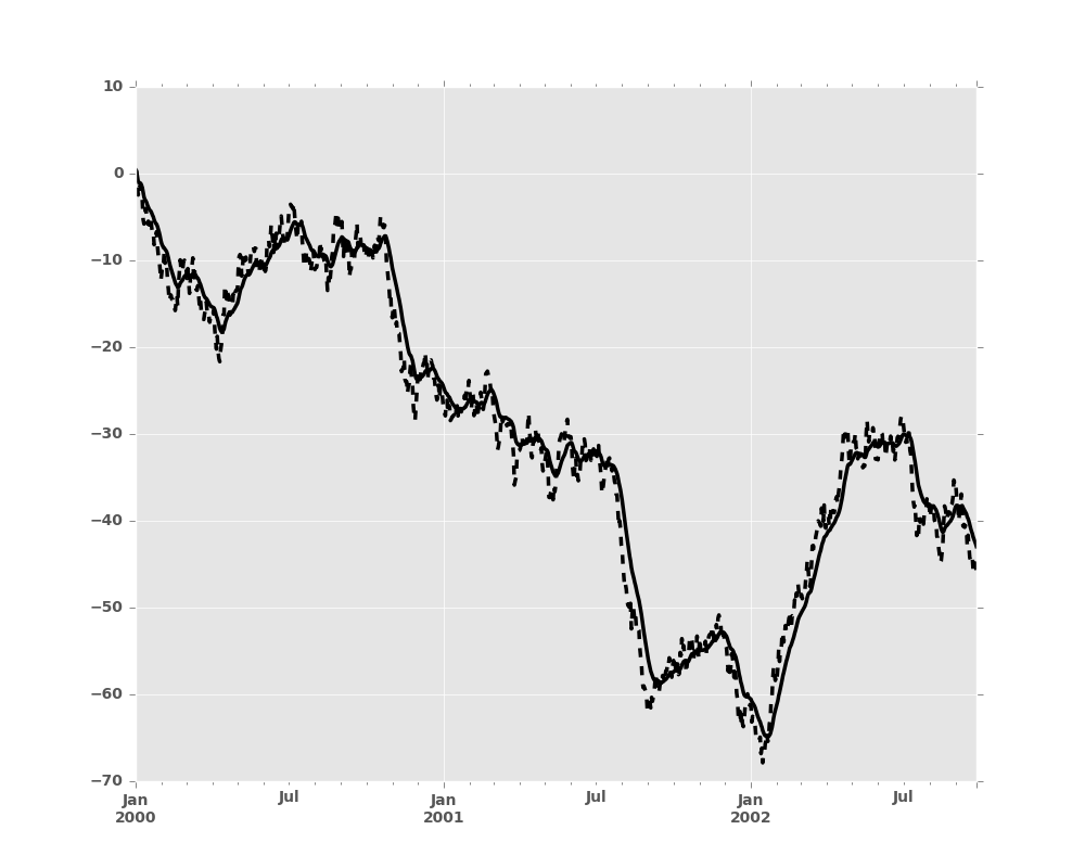
Here is an example for a univariate time series:

In [1]: s.plot(style='k--')
Out[1]: <matplotlib.axes._subplots.AxesSubplot at 0x2b35b9f3e150>

In [2]: s.ewm(span=20).mean().plot(style='k')
Out[2]: <matplotlib.axes._subplots.AxesSubplot at 0x2b35b9f3e150>

EWM has a min_periods argument, which has the same meaning it does for all the .expanding and .rolling methods: no output values will be set until at least min_periods non-null values are encountered in the (expanding) window. (This is a change from versions prior to 0.15.0, in which the min_periods argument affected only the min_periods consecutive entries starting at the first non-null value.)

EWM also has an ignore_na argument, which deterines how intermediate null values affect the calculation of the weights. When ignore_na=False (the default), weights are calculated based on absolute positions, so that intermediate null values affect the result. When ignore_na=True (which reproduces the behavior in versions prior to 0.15.0), weights are calculated by ignoring intermediate null values. For example, assuming adjust=True, if ignore_na=False, the weighted average of 3, NaN, 5 would be calculated as

\[\frac{(1-\alpha)^2 \cdot 3 + 1 \cdot 5}{(1-\alpha)^2 + 1}\]

Whereas if ignore_na=True, the weighted average would be calculated as

\[\frac{(1-\alpha) \cdot 3 + 1 \cdot 5}{(1-\alpha) + 1}.\]

The var(), std(), and cov() functions have a bias argument, specifying whether the result should contain biased or unbiased statistics. For example, if bias=True, ewmvar(x) is calculated as ewmvar(x) = ewma(x**2) - ewma(x)**2; whereas if bias=False (the default), the biased variance statistics are scaled by debiasing factors

\[\frac{\left(\sum_{i=0}^t w_i\right)^2}{\left(\sum_{i=0}^t w_i\right)^2 - \sum_{i=0}^t w_i^2}.\]

(For \(w_i = 1\), this reduces to the usual \(N / (N - 1)\) factor, with \(N = t + 1\).) See Weighted Sample Variance for further details.