5.10 Other useful features

5.10.1 Automatic exclusion of “nuisance” columns

Again consider the example DataFrame we’ve been looking at:

In [1]: df
Out[1]: 
     A      B         C         D
foo    one  0.469112 -0.861849
bar    one -0.282863 -2.104569
foo    two -1.509059 -0.494929
bar  three -1.135632  1.071804
foo    two  1.212112  0.721555
bar    two -0.173215 -0.706771
foo    one  0.119209 -1.039575
foo  three -1.044236  0.271860

Suppose we wish to compute the standard deviation grouped by the A column. There is a slight problem, namely that we don’t care about the data in column B. We refer to this as a “nuisance” column. If the passed aggregation function can’t be applied to some columns, the troublesome columns will be (silently) dropped. Thus, this does not pose any problems:

In [2]: df.groupby('A').std()
Out[2]: 
            C         D
A                      
bar  0.526860  1.591986
foo  1.113308  0.753219

5.10.2 NA and NaT group handling

If there are any NaN or NaT values in the grouping key, these will be automatically excluded. So there will never be an “NA group” or “NaT group”. This was not the case in older versions of pandas, but users were generally discarding the NA group anyway (and supporting it was an implementation headache).

5.10.3 Grouping with ordered factors

Categorical variables represented as instance of pandas’s Categorical class can be used as group keys. If so, the order of the levels will be preserved:

In [3]: data = pd.Series(np.random.randn(100))

In [4]: factor = pd.qcut(data, [0, .25, .5, .75, 1.])

In [5]: data.groupby(factor).mean()
Out[5]: 
[-2.211, -0.987]    -1.461830
(-0.987, -0.0776]   -0.479569
(-0.0776, 0.605]     0.294329
(0.605, 3.357]       1.250221
dtype: float64

5.10.4 Grouping with a Grouper specification

You may need to specify a bit more data to properly group. You can use the pd.Grouper to provide this local control.

In [6]: import datetime

In [7]: df = pd.DataFrame({
   ...:          'Branch' : 'A A A A A A A B'.split(),
   ...:          'Buyer': 'Carl Mark Carl Carl Joe Joe Joe Carl'.split(),
   ...:          'Quantity': [1,3,5,1,8,1,9,3],
   ...:          'Date' : [
   ...:              datetime.datetime(2013,1,1,13,0),
   ...:              datetime.datetime(2013,1,1,13,5),
   ...:              datetime.datetime(2013,10,1,20,0),
   ...:              datetime.datetime(2013,10,2,10,0),
   ...:              datetime.datetime(2013,10,1,20,0),
   ...:              datetime.datetime(2013,10,2,10,0),
   ...:              datetime.datetime(2013,12,2,12,0),
   ...:              datetime.datetime(2013,12,2,14,0),
   ...:              ]
   ...:          })
   ...: 

In [8]: df
Out[8]: 
  Branch Buyer                Date  Quantity
0      A  Carl 2013-01-01 13:00:00         1
1      A  Mark 2013-01-01 13:05:00         3
2      A  Carl 2013-10-01 20:00:00         5
3      A  Carl 2013-10-02 10:00:00         1
4      A   Joe 2013-10-01 20:00:00         8
5      A   Joe 2013-10-02 10:00:00         1
6      A   Joe 2013-12-02 12:00:00         9
7      B  Carl 2013-12-02 14:00:00         3

Groupby a specific column with the desired frequency. This is like resampling.

In [9]: df.groupby([pd.Grouper(freq='1M',key='Date'),'Buyer']).sum()
Out[9]: 
                  Quantity
Date       Buyer          
2013-01-31 Carl          1
           Mark          3
2013-10-31 Carl          6
           Joe           9
2013-12-31 Carl          3
           Joe           9

You have an ambiguous specification in that you have a named index and a column that could be potential groupers.

In [10]: df = df.set_index('Date')

In [11]: df['Date'] = df.index + pd.offsets.MonthEnd(2)

In [12]: df.groupby([pd.Grouper(freq='6M',key='Date'),'Buyer']).sum()
Out[12]: 
                  Quantity
Date       Buyer          
2013-02-28 Carl          1
           Mark          3
2014-02-28 Carl          9
           Joe          18

In [13]: df.groupby([pd.Grouper(freq='6M',level='Date'),'Buyer']).sum()
Out[13]: 
                  Quantity
Date       Buyer          
2013-01-31 Carl          1
           Mark          3
2014-01-31 Carl          9
           Joe          18

5.10.5 Taking the first rows of each group

Just like for a DataFrame or Series you can call head and tail on a groupby:

In [14]: df = pd.DataFrame([[1, 2], [1, 4], [5, 6]], columns=['A', 'B'])

In [15]: df
Out[15]: 
   A  B
0  1  2
1  1  4
2  5  6

In [16]: g = df.groupby('A')

In [17]: g.head(1)
Out[17]: 
   A  B
0  1  2
2  5  6

In [18]: g.tail(1)
Out[18]: 
   A  B
1  1  4
2  5  6

This shows the first or last n rows from each group.

Warning

Before 0.14.0 this was implemented with a fall-through apply, so the result would incorrectly respect the as_index flag:

>>> g.head(1):  # was equivalent to g.apply(lambda x: x.head(1))
      A  B
 A
 1 0  1  2
 5 2  5  6

5.10.6 Taking the nth row of each group

To select from a DataFrame or Series the nth item, use the nth method. This is a reduction method, and will return a single row (or no row) per group if you pass an int for n:

In [19]: df = pd.DataFrame([[1, np.nan], [1, 4], [5, 6]], columns=['A', 'B'])

In [20]: g = df.groupby('A')

In [21]: g.nth(0)
Out[21]: 
     B
A     
1  NaN
5  6.0

In [22]: g.nth(-1)
Out[22]: 
     B
A     
1  4.0
5  6.0

In [23]: g.nth(1)
Out[23]: 
     B
A     
1  4.0

If you want to select the nth not-null item, use the dropna kwarg. For a DataFrame this should be either 'any' or 'all' just like you would pass to dropna, for a Series this just needs to be truthy.

# nth(0) is the same as g.first()
In [24]: g.nth(0, dropna='any')
Out[24]: 
     B
A     
1  4.0
5  6.0

In [25]: g.first()
Out[25]: 
     B
A     
1  4.0
5  6.0

# nth(-1) is the same as g.last()
In [26]: g.nth(-1, dropna='any')  # NaNs denote group exhausted when using dropna
Out[26]: 
     B
A     
1  4.0
5  6.0

In [27]: g.last()
Out[27]: 
     B
A     
1  4.0
5  6.0

In [28]: g.B.nth(0, dropna=True)
Out[28]: 
A
1    4.0
5    6.0
Name: B, dtype: float64

As with other methods, passing as_index=False, will achieve a filtration, which returns the grouped row.

In [29]: df = pd.DataFrame([[1, np.nan], [1, 4], [5, 6]], columns=['A', 'B'])

In [30]: g = df.groupby('A',as_index=False)

In [31]: g.nth(0)
Out[31]: 
   A    B
0  1  NaN
2  5  6.0

In [32]: g.nth(-1)
Out[32]: 
   A    B
1  1  4.0
2  5  6.0

You can also select multiple rows from each group by specifying multiple nth values as a list of ints.

In [33]: business_dates = pd.date_range(start='4/1/2014', end='6/30/2014', freq='B')

In [34]: df = pd.DataFrame(1, index=business_dates, columns=['a', 'b'])

# get the first, 4th, and last date index for each month
In [35]: df.groupby((df.index.year, df.index.month)).nth([0, 3, -1])
Out[35]: 
        a  b
2014 4  1  1
     4  1  1
     4  1  1
     5  1  1
     5  1  1
     5  1  1
     6  1  1
     6  1  1
     6  1  1

5.10.7 Enumerate group items

New in version 0.13.0.

To see the order in which each row appears within its group, use the cumcount method:

In [36]: df = pd.DataFrame(list('aaabba'), columns=['A'])

In [37]: df
Out[37]: 
   A
0  a
1  a
2  a
3  b
4  b
5  a

In [38]: df.groupby('A').cumcount()
Out[38]: 
0    0
1    1
2    2
3    0
4    1
5    3
dtype: int64

In [39]: df.groupby('A').cumcount(ascending=False)  # kwarg only
Out[39]: 
0    3
1    2
2    1
3    1
4    0
5    0
dtype: int64

5.10.8 Plotting

Groupby also works with some plotting methods. For example, suppose we suspect that some features in a DataFrame may differ by group, in this case, the values in column 1 where the group is “B” are 3 higher on average.

In [40]: np.random.seed(1234)

In [41]: df = pd.DataFrame(np.random.randn(50, 2))

In [42]: df['g'] = np.random.choice(['A', 'B'], size=50)

In [43]: df.loc[df['g'] == 'B', 1] += 3

We can easily visualize this with a boxplot:

In [44]: df.groupby('g').boxplot()
Out[44]: 
OrderedDict([('A',
              {'boxes': [<matplotlib.lines.Line2D at 0x2b35becd2550>,
                <matplotlib.lines.Line2D at 0x2b35becdee50>],
               'caps': [<matplotlib.lines.Line2D at 0x2b35becc1510>,
                <matplotlib.lines.Line2D at 0x2b35becd2bd0>,
                <matplotlib.lines.Line2D at 0x2b35bec68fd0>,
                <matplotlib.lines.Line2D at 0x2b35bec35e90>],
               'fliers': [<matplotlib.lines.Line2D at 0x2b35becde890>,
                <matplotlib.lines.Line2D at 0x2b35bec488d0>],
               'means': [],
               'medians': [<matplotlib.lines.Line2D at 0x2b35becde250>,
                <matplotlib.lines.Line2D at 0x2b35bec541d0>],
               'whiskers': [<matplotlib.lines.Line2D at 0x2b35becca2d0>,
                <matplotlib.lines.Line2D at 0x2b35becca1d0>,
                <matplotlib.lines.Line2D at 0x2b35becafed0>,
                <matplotlib.lines.Line2D at 0x2b35becafb50>]}),
             ('B',
              {'boxes': [<matplotlib.lines.Line2D at 0x2b35becd24d0>,
                <matplotlib.lines.Line2D at 0x2b35becf8950>],
               'caps': [<matplotlib.lines.Line2D at 0x2b35bebc3fd0>,
                <matplotlib.lines.Line2D at 0x2b35bebd1950>,
                <matplotlib.lines.Line2D at 0x2b35bed04c50>,
                <matplotlib.lines.Line2D at 0x2b35bed112d0>],
               'fliers': [<matplotlib.lines.Line2D at 0x2b35becf8350>,
                <matplotlib.lines.Line2D at 0x2b35bed11f50>],
               'means': [],
               'medians': [<matplotlib.lines.Line2D at 0x2b35bece7cd0>,
                <matplotlib.lines.Line2D at 0x2b35bed11910>],
               'whiskers': [<matplotlib.lines.Line2D at 0x2b35bebf23d0>,
                <matplotlib.lines.Line2D at 0x2b35bebe4c10>,
                <matplotlib.lines.Line2D at 0x2b35becf8f90>,
                <matplotlib.lines.Line2D at 0x2b35bed04610>]})])

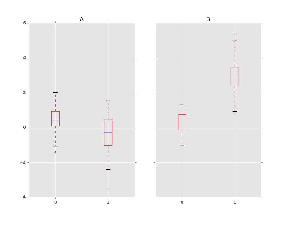
The result of calling boxplot is a dictionary whose keys are the values of our grouping column g (“A” and “B”). The values of the resulting dictionary can be controlled by the return_type keyword of boxplot. See the visualization documentation for more.

Warning

For historical reasons, df.groupby("g").boxplot() is not equivalent to df.boxplot(by="g"). See here for an explanation.